Google Cloud Document AI Layout Parser For RAG Pipelines

Google Cloud Document AI

One of the most frequent challenges in developing retrieval augmented generation (RAG) pipelines is document preparation. Parsing documents, such as PDFs, into digestible parts that can be utilized to create embeddings frequently calls for Python expertise and other libraries. In this blog post, examine new features in BigQuery and Google Cloud Document AI that make this process easier and walk you through a detailed sample.

Streamline document processing in BigQuery

With its tight interaction with Google Cloud Document AI, BigQuery now provides the capability of preprocessing documents for RAG pipelines and other document-centric applications. Now that it’s widely available, the ML.PROCESS_DOCUMENT function can access additional processors, such as Document AI’s Layout Parser processor, which enables you to parse and chunk PDF documents using SQL syntax.

ML.PROCESS_DOCUMENT’s GA offers developers additional advantages:

• Increased scalability: The capacity to process documents more quickly and handle larger ones up to 100 pages
• Simplified syntax: You can communicate with Google Cloud Document AI and integrate them more easily into your RAG workflows with a simplified SQL syntax.
• Document chunking: To create the document chunks required for RAG pipelines, access to extra Document AI processor capabilities, such as Layout Parser,

Specifically, document chunking is a crucial yet difficult step of creating a RAG pipeline. This procedure is made simpler by Google Cloud Document AI Layout Parser. Its examine how this functions in BigQuery and soon illustrate its efficacy with a real-world example.

Document preprocessing for RAG

A large language model (LLM) can provide more accurate responses when huge documents are divided into smaller, semantically related components. This increases the relevance of the information that is retrieved.

To further improve your RAG pipeline, you can generate metadata along with chunks, such as document source, chunk position, and structural information. This will allow you to filter, refine your search results, and debug your code.

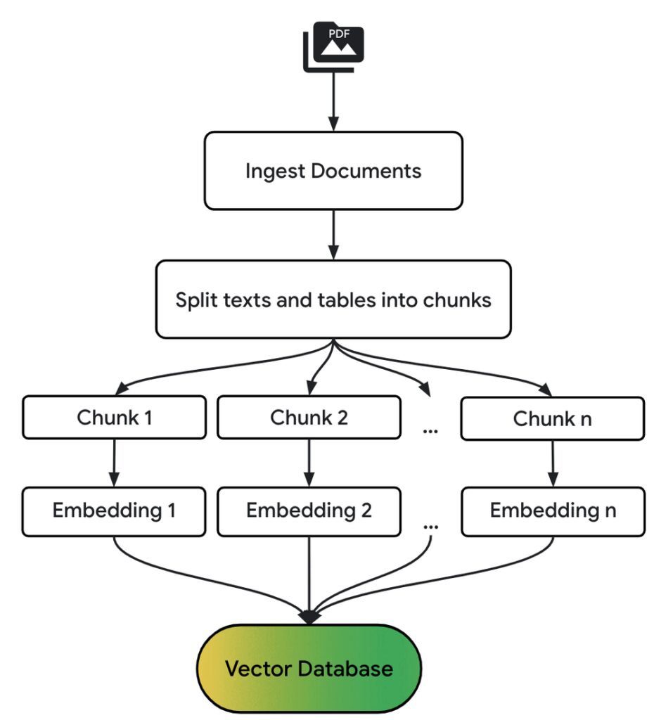
A high-level summary of the preparation stages of a simple RAG pipeline is given in the diagram below:

Build a RAG pipeline in BigQuery

Because of their intricate structure and combination of text, numbers, and tables, financial records such as earnings statements can be difficult to compare. Let’s show you how to use Document AI’s Layout Parser to create a RAG pipeline in BigQuery for analyzing the Federal Reserve’s 2023 Survey of Consumer Finances (SCF) report. You may follow along here in the notebook.

Conventional parsing methods have considerable difficulties when dealing with dense financial documents, such as the SCF report from the Federal Reserve. It is challenging to properly extract information from this roughly 60-page document because it has a variety of text, intricate tables, and embedded charts. In these situations, Google Cloud Document AI Layout Parser shines, efficiently locating and obtaining important data from intricate document layouts like these.

The following general procedures make up building a BigQuery RAG pipeline using Document AI’s Layout Parser.

Create a Layout Parser processor

Make a new processor in Google Cloud Document AI of the LAYOUT_PARSER_PROCESSOR type. The documents can then be accessed and processed by BigQuery by creating a remote model that points to this processor.

Request chunk creation from the CPU

The first step in accessing PDFs in Google Cloud Storage is to create an object table over the earnings statement bucket. After that, give the objects to Google Cloud Document AI using the ML.PROCESS_DOCUMENT method, which will then return the results in BiQuery. Document AI breaks apart the PDF after analyzing it. Returning as JSON objects, the results are simply analyzed to retrieve metadata, such as the page number and source URI.

SELECT * FROM ML.PROCESS_DOCUMENT(
MODEL docai_demo.layout_parser,
TABLE docai_demo.demo,
PROCESS_OPTIONS => (
JSON ‘{“layout_config”: {“chunking_config”: {“chunk_size”: 300}}}’)
);

Parse the document with the ML.PROCESS_DOCUMENT function

Create vector embeddings for the chunks

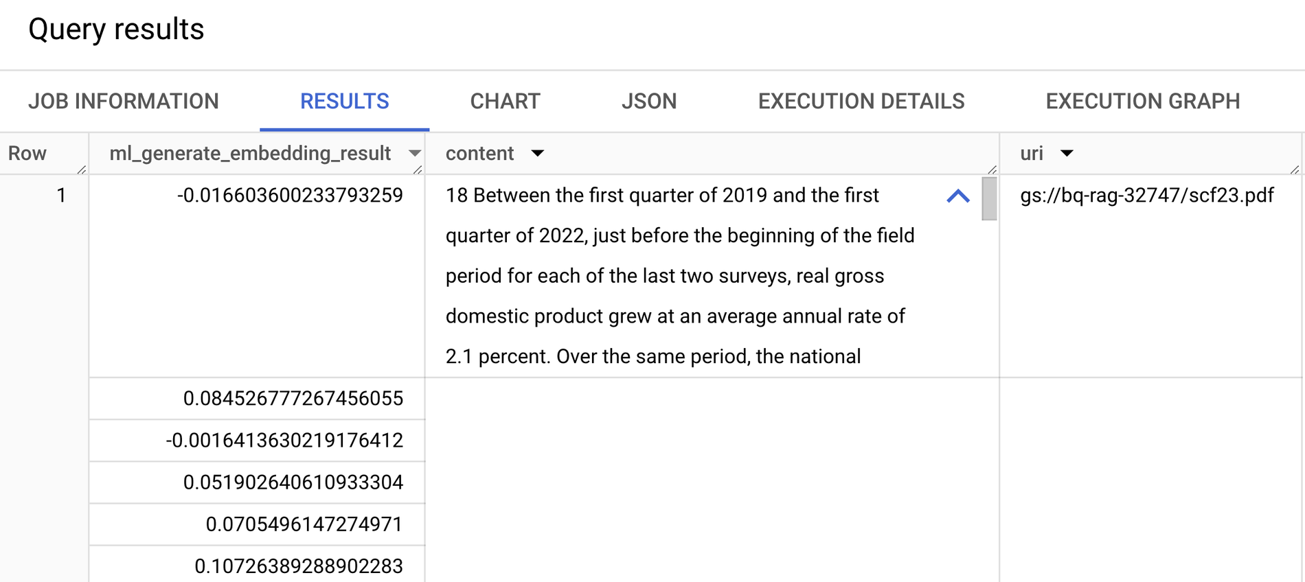
Using the ML.GENERATE_EMBEDDING function, its will create embeddings for every document chunk and write them to a BigQuery table in order to facilitate semantic search and retrieval. Two arguments are required for this function to work:

• The Vertex AI embedding endpoints are called by a remote model.
• A BigQuery database column with information for embedding.

Create a vector index on the embeddings

Google Cloud build a vector index on the embeddings to effectively search through big sections based on semantic similarity. In the absence of a vector index, conducting a search necessitates comparing each query embedding to each embedding in your dataset, which is cumbersome and computationally costly when working with a lot of chunks. To expedite this process, vector indexes employ strategies such as approximate nearest neighbor search.

CREATE VECTOR INDEX my_index
ON docai_demo.embeddings(ml_generate_embedding_result)
OPTIONS(index_type = “TREE_AH”,
distance_type = “EUCLIDIAN”
);

Retrieve relevant chunks and send to LLM for answer generation

To locate chunks that are semantically related to input query, they can now conduct a vector search. In this instance, inquire about the changes in average family net worth throughout the three years covered by this report.

SELECT
ml_generate_text_llm_result AS generated,
prompt
FROM
ML.GENERATE_TEXT( MODEL docai_demo.gemini_flash,
(
SELECT
CONCAT( ‘Did the typical family net worth change? How does this compare the SCF survey a decade earlier? Be concise and use the following context:’,
STRING_AGG(FORMAT(“context: %s and reference: %s”, base.content, base.uri), ‘,\n’)) AS prompt,
FROM
VECTOR_SEARCH( TABLE
docai_demo.embeddings,
‘ml_generate_embedding_result’,
(
SELECT
ml_generate_embedding_result,
content AS query
FROM
ML.GENERATE_EMBEDDING( MODEL docai_demo.embedding_model,
(
SELECT
‘Did the typical family net worth increase? How does this compare the SCF survey a decade earlier?’ AS content
)
)
),
top_k => 10,
OPTIONS => ‘{“fraction_lists_to_search”: 0.01}’)
),
STRUCT(512 AS max_output_tokens, TRUE AS flatten_json_output)
);

The ML.GENERATE_TEXT method then receives the returned chunks, contacts the Gemini 1.5 Flash endpoint, and produces a succinct response to query.

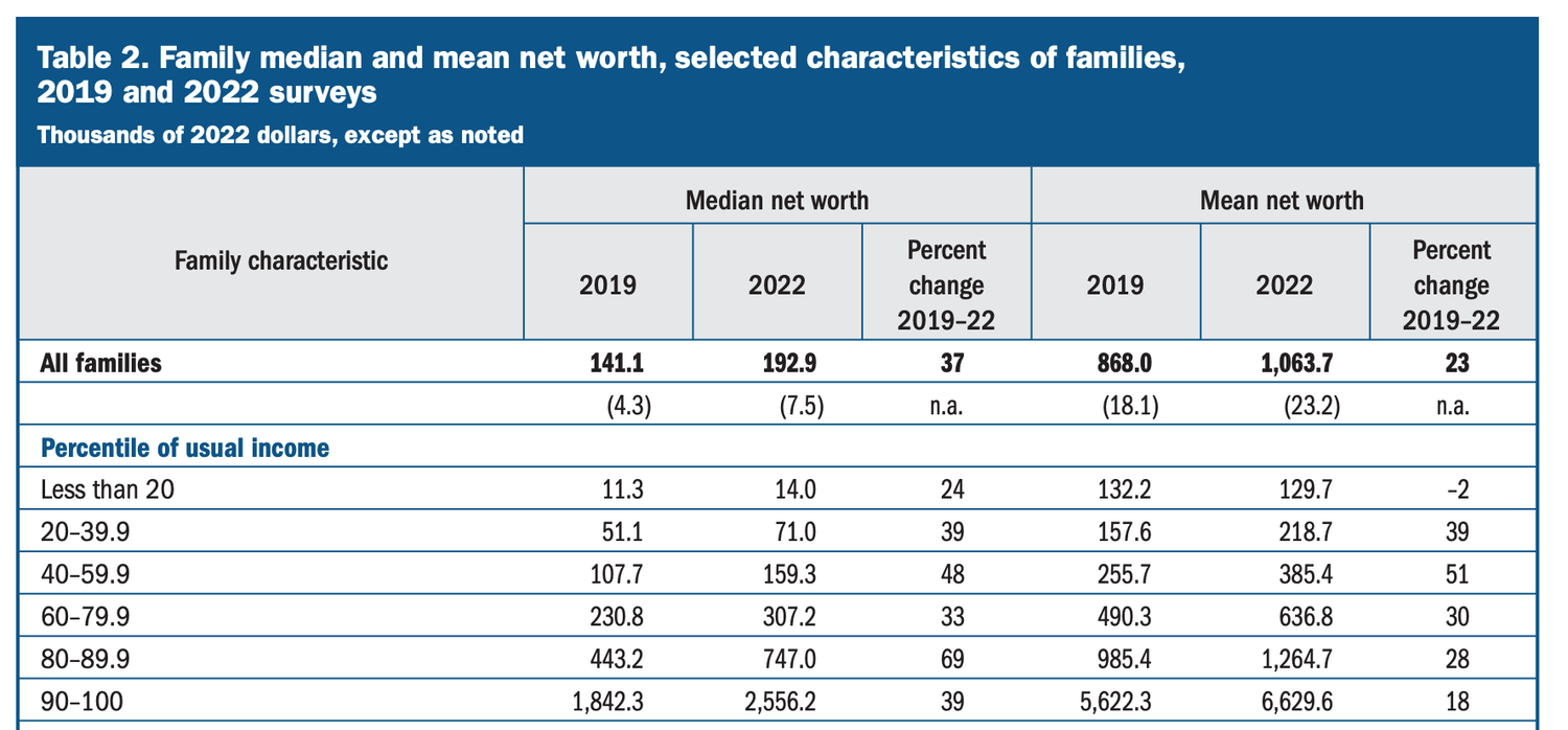
And have an answer: the median family net worth rose 37% between 2019 and 2022, a substantial rise over the 2% decline observed over the same time a decade earlier. If you look at the original paper, you’ll see that this information is located throughout the text, tables, and footnotes areas that are typically difficult to interpret and draw conclusions from together!

Although a simple RAG flow was shown in this example, real-world applications frequently call for constant updates. Consider a situation in which a Cloud Storage bucket receives new financial information every day. Consider using Cloud Composer or BigQuery Workflows to create embeddings in BigQuery and process new documents incrementally to keep your RAG pipeline current. When the underlying data changes, vector indexes are automatically updated to make sure you are always querying the most recent data.