How to Use KV Cache to Maximize LLM Throughput on GPUs in GKE
It can be costly to provide AI foundation models like large language models (LLMs). Organizations require an AI platform that can serve LLMs at scale while minimizing the cost per token because they can’t achieve lower latency without hardware accelerators, and these accelerators aren’t usually used economically. Google Kubernetes Engine (GKE) can assist you in effectively managing workloads and infrastructure by providing capabilities like load balancing and autoscaling.
You must take into account how to serve an application cost-effectively while yet offering the maximum throughput within a given latency bound while integrating LLMs. To assist, Google Cloud developed a performance benchmarking tool for GKE that allows you to evaluate and examine these performance tradeoffs by automating the entire setup process, from cluster construction to inference server deployment and evaluation.
Here are some suggestions to help you get the most out of your NVIDIA GPU providing throughput on GKE. You may set up your inference stack on GKE using data-driven judgments if you combine these suggestions with the performance benchmarking tool. Google Cloud is also discuss how to best utilize a model server platform for a particular workload related to inference.
Decisions about infrastructure
You must choose infrastructure that both matches your model and is economical by providing answers to the following queries:
- Does your model need to be quantized? If yes, which quantization ought you to apply?
- How do you choose the right kind of machine for your model?
- Which GPU ought to be utilized?
Let’s examine these queries in more detail.
Is it appropriate to quantize your model? Which quantization ought to be applied?
KV cache Quantization
The quantization technique uses a lower-precision data type to represent weights and activations, which reduces the amount of accelerator memory needed to load the model weights. Quantization has a smaller memory footprint, which reduces costs and can enhance throughput and latency. However, quantizing a model eventually causes a discernible reduction in accuracy.
FP16 and Bfloat16 quantization, among other quantization methods, use half the memory and, depending on the model, provide about the same accuracy as FP32 (as demonstrated in this work). Most checkpoints from the most recent models have already been released in 16-bit precision. When it comes to model weights, FP8 and INT8 can reduce memory usage by up to 50% (KV cache will still use comparable memory if it isn’t quantized individually by the model server), frequently without sacrificing accuracy.
When quantized to four bits or less, such as INT4 or INT3, accuracy diminishes. Make sure you assess the correctness of the model before applying 4-bit quantization. Additionally, certain post-training quantization methods like Activation Aware Quantization (AWQ) might lessen accuracy loss.
Using our automation tool, you may deploy the model of your choosing with various quantization techniques and assess how well it meets your goals.
First recommendation: To reduce costs and memory usage, use quantization. Use less than 8 bits of precision only after assessing the correctness of the model.
How do you choose the right kind of machine for your model?
The number of parameters in the model and the data type of the model weights can be used to easily determine the machine type you require.
model size (in bytes) = # of model parameters * data type in bytes
Thus, the following would be required for a 7b model utilizing a 16-bit precision quantization approach, such FP16 or BF16:
7 billion * 2 bytes = 14 billion bytes = 14 GiB
Likewise, for a 7b model in 8-bit precision such as FP8 or INT8, you’d need:
7 billion * 1 byte = 7 billion bytes = 7 GiB
Google Cloud has used these recommendations to indicate how much accelerator memory you could require for a few common open-weight LLMs in the table below.
| Models | Model Variants(# of parameters) | Model Size (GPU memory needed in GB) | ||
| FP16 | 8-bit precision | 4-bit precision | ||
| Gemma | 2b | 4 | 2 | 1 |
| 7b | 14 | 7 | 3.5 | |
| Llama 3 | 8b | 16 | 8 | 4 |
| 70b | 140 | 70 | 35 | |
| Falcon | 7b | 14 | 14 | 3.5 |
| 40b | 80 | 40 | 20 | |
| 180b | 360 | 180 | 90 | |
| Flan T5 | 11b | 22 | 11 | 5.5 |
| Bloom | 176b | 352 | 176 | 88 |
Note: This table is meant only to serve as a guide. The number of parameters listed in the model name, such as Llama 3 8b or Gemma 7b, may not match the actual number of parameters. The Hugging Face model card page contains the precise amount of parameters for open models.
Selecting an accelerator that devotes up to 80% of its RAM to model weights while keeping 20% for the KV cache a key-value cache that the model server uses to generate tokens quickly is recommended as best practice. You can need 19.2 GB for model weights (24 * 0.8) on a G2 machine type with a single NVIDIA L4 Tensor Core GPU (24GB), for instance.
You may require up to 35 percent for the KV cache, depending on the length of the token and the quantity of requests fulfilled. You will need to set aside even more memory for the KV cache and anticipate that it will take up the majority of memory use for very long context lengths, such as 1 million tokens.
Second Recommendation: Select your NVIDIA GPU according to the model’s memory specifications. Use tensor parallelism in conjunction with multi-GPU sharding when one GPU is insufficient.
Which GPU ought to be utilized?
NVIDIA GPU-powered virtual machines (VMs) are widely available from GKE. How do you choose the best GPU to run your model on?
It should be noted that you can leverage structural sparsity to increase performance with the A3 and G2 virtual machines. There is sparsity in the values displayed. The mentioned specs are half as high without sparsity.
Three distinct dimensions can be used to limit throughput and latency depending on the features of a model:
- GPU memory (GB / GPU) could be a limiting factor in throughput because it stores the KV cache and model weights. Throughput is increased by batching, but ultimately the KV cache growth reaches its memory limit.
- GPU HBM speed (GB/s) may be a limiting factor in latency: depending on memory capacity, model weights and KV cache state are read for each and every token that is generated.
- GPU FLOPS may limit latency for larger models: The GPU FLOPS is required for Tensor computations. Increased attention heads and concealed layers signify increased FLOPS utilization.
When selecting the best accelerator to meet your latency and throughput requirements, take these factors into account.
The throughput/$ of G2 and A3 for the Llama 2 7b and Llama 2 70b models are contrasted below. Normalized throughput/$ is used in the chart, with G2’s performance set to 1 and A3’s performance measured against it.

At larger batch sizes, the Llama 2 7b model outperforms A3 in terms of throughput/$, as seen by the graph on the left. The graph on the right-hand side demonstrates that A3 outperforms G2 in terms of throughput/$ at larger batch sizes when employing several GPUs to service the Llama 2 70b model. This also applies to other models with comparable sizes, such as the Falcon 7b and Flan T5.
Selecting the GPU machine of your choice and utilizing our automation tool to build GKE clusters will allow you to run the model and model server of your choice.
Third recommendation: if the delay is tolerable, use G2 for models with 7b parameters or fewer for better price/performance. For larger models, use A3.
Optimize model servers
Batching
HuggingFace TGI, JetStream, NVIDIA Triton and TensorRT-LLM, and vLLM are among the model servers that can serve your LLM on GKE. The overall performance of your LLM can be enhanced by certain model servers’ support for significant improvements such batching, PagedAttention, quantization, etc. When preparing the model server for your LLM workloads, consider these questions.
How can you optimize for use cases that are more output-heavy than input-heavy?
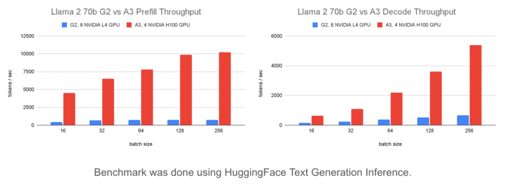
Prefill and decode are the two stages of LLM inference.
- The prefill stage creates the KV cache and processes the tokens in a prompt in parallel. In comparison to the decode phase, it is a reduced latency and higher throughput operation.
- New tokens are generated sequentially depending on the KV cache state and the previously generated tokens during the decode phase, which comes after the prefill phase. In comparison to the prefill phase, this operation has a higher latency and a lower throughput.
Your use-case will determine whether you have a longer output (content production) or a longer input (summarization, classification), or a roughly equal distribution of the two.
Below is a comparison of the prefill throughput for G2 and A3.

The graphs demonstrate that at 5.5 times the cost, A3 offers 13.8 times the prefill throughput of G2. A3 will therefore offer 2.5 times greater throughput per $ if your use case involves a longer input length.
The benchmarking tool allows you to simulate various input/output patterns that suit your demands and verify their effectiveness.
Fourth recommendation: On models with a substantially longer input prompt than output, use A3 for better price/performance. Examine your model’s input/output pattern to determine which infrastructure will offer the highest value in terms of both cost and performance for your use case.
What impact does batching have on output?
Since batch requests use more GPU memory, HBM bandwidth, and GPU FLOPS without increasing costs, they are crucial for obtaining higher throughput.
The impact on throughput and delay is demonstrated in the comparison of various batch sizes utilizing static batches and fixed input/output lengths below.

The graph on the left illustrates how throughput on a Llama 2 70b model delivered on A3 may be enhanced by up to 8x by raising batch size from 16 to 256. On G2, it can increase throughput by up to 4 times.
The impact of batching on latency is depicted in the graph on the right. There is a 1,963 ms increase in latency on the G2. However, latency rises by 155 ms on A3. This demonstrates that, up until the batch size reaches the compute-bound threshold, A3 can handle increasing batch sizes with little increase in latency.
In order to determine the optimal batch size, you must increase the batch size until you reach your latency target or until the throughput stops improving.
Using the benchmarking tool’s monitoring automation, you can keep an eye on your model server’s batch size. Then, you can use that to determine what the perfect batch size is for your system.
Fifth recommendation: Increase throughput by using batching. The ideal batch size is determined by the latency you require. Select A3 to reduce latency. In situations where a little bit of delay is acceptable, go with G2 to save money.


